Quantum Computing #5: Quantum Teleportation

Previously:

Introduction
Single Qubit Gates
Multiple Qubit Gates
Measurement & Review
Superdense Coding

Beam Me Over

If you took the time to digest the previous article on the Superdense Coding protocol, you'll find comparatively few surprises in this one. Remember how two entangled qubits were initially prepared in a special Bell State; then one was sent directly to Bob, while Alice processed the second to encode two classical bits of data. Later, Bob successfully decoded those two classical bits. Didn't it seem to you as if Alice somehow reached across the divide, fiddling with the independent states of both qubits, using some kind of spooky action at a distance?

The Quantum Teleportation protocol is a very similar trick. In fact, you could say that it's exactly the same trick, but performed in reverse. This time, using the magic of the entangled qubit pair, and precisely the same set of quantum gates as before, Alice will teleport to Bob the full state vector of an arbitrary third qubit - using only two classical bits of information.

There are three preliminary, new, key concepts - all related to the notion of measurement - that we'll need in order to investigate and explain the Quantum Teleportation phenomenon today. The first of these is:

The Measurement Basis

Specifically, the performance of a measurement in an arbitrary basis. Recall that in part one we said the labels 0 and 1 might represent unit steps in some arbitrary x- and y-directions. When later we made a measurement in the computational basis, we were in effect holding up a filter, constraining the result to be either 0 or 1 in this sense. But we are free to change this basis!

To take a brief physical detour, suppose our qubit is a photon, and measurement involves holding up a pair of polarized sunglasses, either horizontally or vertically, to see whether or not the photon gets through the lens. We know there's a 50-50 chance it that will, simply because holding up two such identical and overlapping lenses, one horizontally and one vertically, will prevent any photons from getting through. But what's to prevent us holding our sunglasses at ±45° to the horizontal?

Nothing. All we're doing is changing the basis of measurement, from the original computational basis, i.e. horizontal 0 or vertical 1, to this new one, where perhaps 0' and 1' mean pointing respectively up or down at 45°. From the diagram we see these new basis vectors can be expressed readily in terms of the originals, like this:

0' = (0+1)/√2,
1' = (0-1)/√2.

But this is precisely the state transformation performed by the Hadamard gate. Now we can see that it corresponds to a particular reflection, in a line at 22½° to our basis 0 vector (the light grey line in the diagram is this axis of symmetry). Incidentally this illustrates nicely why the Hadamard gate, like any reflection, is its own inverse; since we also have these perfectly symmetrical equations,

0 = (0'+1')/√2,
1 = (0'-1')/√2.

And just as 0' and 1' give us an alternative orthonormal basis for measuring single-qubit states previously expressed in terms of our original computational basis 0 and 1, so too are there any number of alternative bases for a given multi-qubit measurement. One important example in 2-qubit systems is:

The Bell Basis

This is today's new concept number two. Starting from any given 2-qubit computational basis 00, 01, 10 and 11, the Bell basis can be defined as

B₀ = (00+11)/√2,
B₁ = (10+01)/√2,
B₂ = (00-11)/√2,
B₃ = (10-01)/√2.

Notice that these four are exactly the states that Alice prepared last time, in the Superdense Coding protocol, by inserting either an X or a Z gate (or both, or neither) into the path of the top qubit of a pair - an entangled pair, which happened to have been prepared in a certain special initial state. We now recognise that state as B₀ = (00+11)/√2.

Exactly as before, it's easy to check by substitution that we can express the Bell state mapping the other way round, for convenience in our subsequent conversions:

00 = (B₀+B₂)/√2,
01 = (B₁-B₃)/√2,
10 = (B₁+B₃)/√2,
11 = (B₀-B₂)/√2.

Partial Measurements

Our third and final new concept of the day is that of a partial measurement. What happens to a composite, multi-qubit state when we perform measurements upon some, but not all, of its constituent qubits? Answer: measured qubits collapse into appropriate basis states in accordance with the probabilities in effect, while unmeasured ones continue in renormalized superpositions.

Take for example the 2-qubit state (a, b, c, d) = a00 + b01 + c10 + d11, and suppose that we perform a measurement, in the computational basis, on its first qubit. Then the probability of getting a result of 0 is simply the sum of the probabilities of getting either 00 or 01 from a full, 2-qubit measurement. Similarly, the probability of a 1 is just the sum for 10 and 11:

prob(0?) = prob(00) + prob(01) = |a|² + |b|²,
prob(1?) = prob(10) + prob(11) = |c|² + |d|².

Okay, that tells us everything we can ever know about the first qubit. What can we say about the posterior state of the second qubit, i.e., its state after this partial measurement? We can answer this by rewriting the original state, collecting terms involving a result of 0 or 1 for the first qubit measurement:

(a, b, c, d) = a00 + b01 + c10 + d11 = 0 (a0 + b1) + 1 (c0 + d1).

This lets us read off the result. If the measurement yielded 0 for the first qubit, then the second qubit is now in the state indicated by a0 + b1, which of course we must renormalize as usual:

(a0 + b1) / √(|a|² + |b|²).

Similarly, a measurement of 1 for the first qubit implies that the second is now in this state:

(c0 + d1) / √(|c|² + |d|²).

Quantum Teleportation

Now we finally have enough background to understand the Quantum Teleportation protocol, which is illustrated in the diagram below. Alice starts with an arbitrary qubit state which I've called ψ, pronounced sigh, out of deference to 86 years of quantum mechanics... sorry about that!

So Alice starts with ψ = (a, b) = a0 + b1, where |a|² + |b|² = 1. This is the state she wants to communicate to Bob; and she also has access to one qubit of an entangled pair, previously prepared in the state

B₀ = (00+11)/√2.

She now performs the "decoding" second half of the Superdense Coding protocol on her two qubits. So that's a cNOT, followed by a Hadamard on the first qubit, then a 2-qubit measurement. Remember, this was the operation performed by Bob last time, and it yields a couple of classical bit results. We've shown these as thick double wires, intended to give the impression of big, strong, macroscopic classical logic levels, insusceptible to decoherence. This decoding operation is actually termed a measurement in the Bell basis. Furthermore, in this setup it's a partial measurement. Recall that we are dealing with a system of three entangled qubits, but measuring only two of them. The third, the bottom one in the diagram, is simply transmitted directly to Bob.


Now Bob examines those two classical bits of data he's received from Alice, and uses them to decide which, if any, of his decoding X and Z gates to apply. His logic is exactly the reverse of the "encoding" step used in the first half of the Superdense Coding protocol. And that's all there is to the Quantum Teleportation protocol; the output that Bob ultimately obtains is identical to Alice's initial, arbitrary state ψ.

I Don't Believe You

And who can blame you! Okay, but be warned: I'll be renormalizing throughout today, so as to avoid any sleight-of-hand accusations. So let's start with the initial state of the 3-qubit system,

(a0 + b1)(00 + 11) / √2 = [a (000 + 011) + b (100 + 111)] / √2.

Alice begins by passing the first two qubits through a cNOT gate. This flips the state of the second qubit in the last two terms, i.e., those where the first "control" qubit is 1, resulting in the state

[a (000 + 011) + b (110 + 101)] / √2.

Next she passes the first qubit through a Hadamard. The effect of this is to replace every initial 0 with (0+1)/√2, and every initial 1 with (0-1)/√2. Collecting terms and combining the √2 divisors, we now have the state

[a (000 + 011 + 100 + 111) + b (001 + 010 - 101 - 110)] / 2.

This is the point at which Alice performs the partial measurement upon the first two qubits. The probability of her getting a result of 00 is

prob(00?) = prob(000) + prob(001) = (|a|² + |b|²) / 4 = ¼,

since |a|² + |b|² = 1. And in fact if you work out the remaining probabilities for results 01, 10 and 11, they all turn out to be ¼. Think about that - the measurement outcome is absolutely random, and completely independent of the particular state of the input qubit ψ! This happens because - thanks to the cNOT and H gates - we are performing the measurement in the Bell basis, and not in the original computational basis where we started.

Fascinating as this detail may be, nevertheless it's not quite what we're after here. We want to know the posterior state of the third qubit. This does depend critically upon the particular 2-bit classical result just obtained, so just as in the Superdense Coding protocol, we now have four distinct cases to consider.

________

Case 00: keeping only the 000 and 001 terms from our state expression and renormalizing, we obtain the state received by Bob:

00 (a0 + b1) = 00 ψ.

That's the magic of quantum teleportation! Without doing anything further, Bob knows from the classical measurement 00 that his third qubit is already in Alice's initial state, ψ.

________

Case 01: keeping only the 010 and 011 terms from our state expression, and renormailzing, we obtain the state received by Bob:

01 (a1 + b0).

Notice however that the 1 bit in the classical measurement result activates the X gate in Bob's decoding circuit, causing a logical inversion of the third qubit, and a final state of

01 (a0 + b1) = 01 ψ.

Again, Bob has successfully received Alice's full state ψ in that third qubit.

________

Case 10: keeping only the 100 and 101 terms from our state expression, and renormailzing, we obtain the state received by Bob:

10 (a0 - b1).

Notice however that the 1 bit in the classical measurement result activates the Z gate in Bob's decoding circuit, causing a sign change in the second basis component of the third qubit, and a final state of

10 (a0 + b1) = 10 ψ.

Again, Bob has successfully received Alice's full state ψ in that third qubit.

________

Case 11: keeping only the 110 and 111 terms from our state expression, and renormailzing, we obtain the state received by Bob:

11 (a1 - b0).

This time both bits in the classical measurement result are 1, so this state becomes subjected to both the full logical inversion and the phase (sign) change, and the final 3-qubit state is

11 (a0 + b1) = 11 ψ.

So in all four cases - in other words, regardless of the outcome of the partial measurement operation - Bob has successfully received Alice's full state ψ in the third qubit.

________

Interactive Demo

Once again Brad Rubin steps up with the Wolfram Demonstrations Project simulation of the Quantum Teleportation protocol, a model of clarity:


This ingenious demo lets you vary both the arbitrary input state ψ, by dragging the indicator point in the upper graph, and the 2-qubit partial measurement result, using the radio buttons below it. Intermediate states of the 3-qubit system are displayed as continuously updated column vectors.

Picture of Star Trek transporter chamber from Wikipedia.

Quantum Computing #4: Superdense Coding

Previously:

Introduction
Single Qubit Gates
Multiple Qubit Gates
Measurement & Review

Note: Last week's removal of Greek lettering and matrices has proved too popular to ignore, all feedback being either positive or neutral, so I'll continue using this "new" notation wherever possible.

Breaking News! A single qubit can transmit two full classical bits of information.

Not on its own, though. We can only ever encode one single classical bit of information into a solitary, unentangled qubit. But when we have access to an entangled pair, we can choose to send one unmodified to our intended recipient, and encode a full two classical bits into the other. To see how, we'll have to examine four quite similar quantum circuits. And we'll need the help of a new single-qubit gate we haven't met before:

The Z Gate

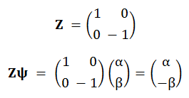
Like its partner the X gate, Z is a kind of inverter. It maps the input qubit state (a, b) to (a, -b). We say that it inverts the phase of the second basis vector. For the sake of completeness alone, here is its matrix representation:

Preparing the Bell State

The two qubits that we'll be using to perform the superdense coding trick have to be entangled, so first let's see how to achieve that. One way is to prepare them both initially in the 0 state. Next, we pass the first qubit of the pair through a Hadamard gate. Finally, we use the output of the H gate as the control input of a controlled-NOT gate, conditionally inverting the second qubit:

The H gate converts the first 0 into 0+1, where I'm going to use '+' and '-' to mean "normalized vector sum" and "normalized vector difference", just to get rid of all the visual noise generated in the calculations by incessant divisions by √2. Since the second qubit remains at 0, the combined state after the H gate is 00+10. Nothing strange about this so far; all it says is that a measurement on the first qubit will yield either 0 or 1, each with 50% probability, while a measurement on the second qubit will still yield 0, with 100% certainty.

Next, the qubits arrive at the cNOT gate. This has no effect upon the first part 00 of the superposition, since there the control (first) qubit is 0. However the second part, 10, has a 1 in the control bit position, causing the cNOT gate to invert the second qubit. The combined state at the output of the cNOT gate is therefore 00+11.

This is termed a Bell State, and it's actually a fairly remarkable state when you think about it. It says that the qubit pair is in a perfectly balanced superposition of the 00 and 11 states. Expressed as a sequence of renormalized amplitudes, it is

(a, b, c, d) = (1/√2, 0, 0, 1/√2)

Since |a|² = |d|² = ½, while |b|² = |c|² = 0, this says that a measurement is equally likely (50%) to yield 00 or 11, and to do so absolutely randomly; but it can never yield 01 or 10. Now if you measure just one of the qubits, whatever result you obtain, 0 or 1, you'll get exactly the same outcome when you measure the second qubit. Even if it's hours or years later, miles or light years away.

Encoding and Decoding

Remember that both Hadamard gates and inverters are their own inverses. If we were to make a mirror image of the above diagram and then join the two together, our final output state would be the same as the originally prepared 00, with probability 100%. This mirror image decoder is shown below, if we temporarily ignore the "?" gate (imagine it to be just a quantum wire, or an Identity gate I):

Suppose Alice is in charge of the "?" box, and Bob is performing the final measurements. Alice wants to send 2 classical bits of data to Bob, but she's only allowed to operate upon the first of the two qubits (the top one in the diagram) to do it. What should she put in the "?" box?

Well, if the bits she wants to send are 00, then she need apply nothing but a simple quantum wire, since we've just seen that this will result in Bob's measurements yielding the result 00 with 100% certainty. In the more general case, she needs to examine both of the classical bits that she wants to send. If the first is 1, then she should add our new friend the Z gate in place of the "?". If the second is 1, she adds an X. Note that if both bits are 1, she will now have added both a Z and a following X.

00 → I
01 → Z
10 → X
11 → Z followed by X

And that's all there is to the Superdense Coding Protocol. With those arrangements in place, Bob's measurements will always yield, with 100% certainty, the particular combined state 00, 01, 10, or 11 that Alice wanted to send him.

I Don't Believe You

No, you'd be mad to, unless you're already a QC expert! We'll go through the four cases individually in detail. Remember, the starting point for Alice is in each case the Bell State 00+11. It will also be useful to remember the reversibility of the H gate. Just as it converts basis states 0 and 1 respectively into their sum 0+1 and difference 0-1, so when presented with a sum 0+1 at its input, does it output 0; and with a difference 0-1, output 1.

Case 00: We already established, using an argument based on considerations of symmetry, the correct operation of the circuit for this first case. Still, it's worth running through the detailed sequence of decoding steps, since these are the same for all subsequent cases. So: Alice does nothing to the 00+11 state, which is then passed immediately into the second cNOT gate. This has no effect on the 00 portion of its input, but changes the 11 part (because the first, control bit is 1) into 10. The cNOT output is therefore 00+10. The first of these qubits, 0+1, is fed to the second Hadamard, which as mentioned above, converts it to 0. Therefore, the final 2-qubit output is 00, with probability 100%.

Case 01: Alice inserts an X gate in the path of the first qubit, converting the initial 00+11 to 10+01. The cNOT changes this to 11+01, feeding the first qubit 1+0 into H, which outputs 0. Therefore, the final 2-qubit output is 01, with probability 100%.

Case 10: Alice inserts a Z gate in the path of the first qubit, converting the initial 00+11 to 00-11. The cNOT changes this to 00-10, feeding the first qubit 0-1 into H, which outputs 1. Therefore, the final 2-qubit output is 10, with probability 100%.

Case 11: Alice inserts both a Z and a following X into the path of the first qubit, converting the initial 00+11 first to 00-11 as in the previous case, then to 10-01. The cNOT changes this to 11-01, feeding the first qubit 1-0 into H, which outputs 1. Therefore, the final 2-qubit output is 11, with probability 100%.

Quantum Erat Demonstrandum!

The second most surprising thing about Superdense Coding - other than the fact that in reality, it works exactly as advertised! - is the time it took to get itself discovered. The whole subject of Quantum Mechanics was kicked off by Werner Heisenberg in 1925, with Quantum Computing eventually appearing with Richard Feynman in 1982; yet it was a further ten years after that before the definitive Bennett & Wiesner paper appeared, noting that certain "EPR" (Einstein-Podolsky-Rosen) states "allow two bits to be encoded reliably in one spin-½ particle..."

Interactive Demo

The Wolfram Demonstrations Project contains a great interactive demo of the Superdense Coding protocol, one of several contributed by Brad Rubin. This varies a little from the our example, specifically in the order of the X and Z gates during the 11 case, but the difference vanishes during final measurement. You interact with it by downloading the Computable Document Format (CDF) Player, and optionally the Superdense Coding demo file itself, which looks like this:


As you can see, it displays all the intermediate states of the qubits during this quantum computation - and fully normalized, hence all the "1/√2"s.

Footnote

In this series I've been avoiding discussion about the physical realisation of qubits, but the day after I posted this comment on digital simulator Logicly's Facebook page...

Has anyone ever asked for a quantum circuit version? You seem to have all the component building and layout logic that would require. Qubit signals: rather than boolean, these would be pairs of complex numbers (or quadruples of floats), and there would be a "measurement" gate with a classical boolean 0 or 1 output. Now seems a good time to start training up on these!

... noted futurologist and SF author Charles Stross predicted room temperature quantum computing on integrated circuitry within 5 to 20 years, based on a fascinating discovery about silicon carbide. My guess is that many more suitable materials will be discovered quite soon, making available QC technologies that will have absolutely no trouble attracting capital investment at the left hand edge of that range.

Next time: Quantum Teleportation.

Quantum Computing #3: Measurement + Review

Previously:

Introduction
Single Qubit Gates
Multiple Qubit Gates

Why One?

When we looked at the state of a single qubit, ψ = α0 + β1, we noted that this vector had to be of unit length, a stipulation encoded in the normalization condition |α|² + |β|² = 1. Similarly when we extended to a 2 qubit system, ψ = α00 + β01 + γ10 + δ11, we maintained the analogous constraint |α|² + |β|² + |γ|² + |δ|² = 1. This was accomplished by only ever applying so-called unitary (magnitude-preserving) matrix operations to the current state.

The reason for this has to do with the method of getting results out of a quantum computer, which is done by the process of measurement. The outcome of a given measurement operation can be any one of the system's basis states. that is, it will be either 0 or 1 for a single qubit system; 00, 01, 10 or 11 for a 2-qubit system; and so on. Which of the basis states actually gets detected depends upon various probabilities, and in fact these probabilities are just |α|², |β|², etc.

So to clarify, when we perform an operation of measurement in the computational basis on an n-qubit system, we are effectively forcing the state vector to settle into one of its 2ⁿ basis states. Taking the 2-qubit case as an example, the result of the measurement will be either

00 with probability |α|²,
01 with probability |β|²,
10 with probability |γ|², or
11 with probability |δ|².

Since these are the only possible outcomes, it's easy to see why the sums of the squares of the coefficients α, β, γ and δ must be unity - after all, there's a 100% probability the outcome will be one of these states!

Destructive Read

The measurement operation irrevocably destroys the previously existing superposition of states, leaving only the single basis state that is the result of the measurement. This means that the original state can never be directly observed. All that we can ever know about it comes from the results of destructive read operations.

For example, suppose we prepare a qubit in the 0 state, then immediately make a measurement. What will the outcome be? Well, the qubit state is ψ = 0 = α0 + β1, where α = 1 and β = 0. Measurement will deliver either the state 0 with probability |α|² = 1 (100% certainty), or else the state 1 with probability |β|² = 0 (0% impossibility). So far, so perfectly common sensible...

Now, suppose we pass the qubit through a Hadamard gate before making the measurement. The diagram below shows this new process:


The output of the H gate prior to measurement is ψ = α0 + β1, where α = β = 1/√2; so we have |α|² = |β|² = ½. In other words, the measurement is equally likely to deliver either 0 or 1; the probability of each is 50%. But regardless of which outcome is observed, the state of the qubit after the measurement is just that observed basis state; the original superposition of equal quantities 0 and 1 has been obliterated by the measurement operation.

Review

More than one reader still finds too much unfamiliar notation in my little introductory series, so here's a quick redux of the story so far, without all the matrices and Greek letters...

Qubits without Greek

A single qubit can be represented as an ordered pair of numbers (a, b), where |a|² + |b|² = 1. In this scheme, the pair (1, 0) represents the classical logical 0, while (0, 1) represents classical 1:

(1, 0) = 0
(0, 1) = 1

Similarly, an entangled pair of qubits can be represented as an ordered sequence (a, b, c, d), where |a|² + |b|² + |c|² + |d|² = 1, and the four particular values (1, 0, 0, 0), (0, 1, 0, 0), (0, 0, 1, 0) and (0, 0, 0, 1) stand respectively for the classical states 00, 01, 10 and 11:

(1, 0, 0, 0) = 00
(0, 1, 0, 0) = 01
(0, 0, 1, 0) = 10
(0, 0, 0, 1) = 11

An entangled triplet is represented as a sequence of eight amplitudes (a, b, c, d, e, f, g, h), where |a|² + |b|² + |c|² + |d|² + |e|² + |f|² + |g|² + |h|² = 1, and the following correspondence holds between basis and classical states:

(1, 0, 0, 0, 0, 0, 0, 0) = 000
(0, 1, 0, 0, 0, 0, 0, 0) = 001
(0, 0, 1, 0, 0, 0, 0, 0) = 010
(0, 0, 0, 1, 0, 0, 0, 0) = 011
(0, 0, 0, 0, 1, 0, 0, 0) = 100
(0, 0, 0, 0, 0, 1, 0, 0) = 101
(0, 0, 0, 0, 0, 0, 1, 0) = 110
(0, 0, 0, 0, 0, 0, 0, 1) = 111

When our quantum computers are big enough to contain n entangled qubits, there will be 2ⁿ coefficients or "amplitudes" a, b, c, ..., and still the sum of all their squares will be 1.

Quantum Gates without Matrices

Like classical logic gates, quantum gates are defined by the operation they perform upon their inputs. In the case of a single qubit gate, we could say the input state (a, b) results in the output (a', b'):

(a, b) → (a', b'),

where of course |a'|² + |b'|² = 1. The single-qubit gates we looked at in part 1 were: firstly the quantum wire I, which transmits the input qubit unaltered:

(a, b) → (a, b)

secondly the quantum inverter or NOT gate X, which swaps the two amplitudes of its single-qubit input, and so in particular, converts classical 0 to 1 and vice-versa:

(a, b) → (b. a)

(1, 0) → (0, 1) = 0 → 1
(0, 1) → (1, 0) = 1 → 0

and lastly, for a bit of quantum exclusivity, the Hadamard gate H, which can combine pure basis states:

(a, b) → ((a+b)/√2, (a-b)/√2)

You might find this last operation written without the √2 scale factors, particularly in multi-step quantum computations, when it is common to roll up such adjustments into a single normalization following the final step of the calculation:

(a, b) → (a+b, a-b)

The only multiple-qubit gate we've seen so far is the controlled-NOT or cNOT gate, which swaps the last two amplitudes of its entangled input qubit pair:

(a, b, c, d) → (a, b, d, c)

By explicitly tracing through the details of the four transitions, we found that this twist corresponded to an inversion of the second qubit, if and only if the first qubit was 1:

(1, 0, 0, 0) → (1, 0, 0, 0) = 00 → 00;
(0, 1, 0, 0) → (0, 1, 0, 0) = 01 → 01;
(0, 0, 1, 0) → (0, 0, 0, 1) = 10 → 11;
(0, 0, 0, 1) → (0, 0, 1, 0) = 11 → 10.

Measurement

Finally, in the first half of this article, we have just covered the question of getting results out of the qubit complex. When you perform a measurement in the computational basis, the single qubit (a, b) will deliver a result of either (1, 0) = 0, with probability |a|², or else (0, 1) = 1, with probability |b|². The qubit will also adopt that measured state, from the point of the measurement onwards; having collapsed into probabilities, there now remains no trace of the original state amplitudes (a, b).

To take a numerical example, the (unknowable) initial state of the qubit might be (a, b) = (+0.8, -0.6). Now suppose a measurement is performed on this qubit. The outcome will be either 0, with a probability of |a|² = 0.8² = 64%, or else 1, with a probability of |b|² = 0.6² = 36%. Notice that the two outcomes have probabilities adding up to 100%, and that between them, they exhaust all the possibilities.

A similar measurement upon a qubit pair in the state (a, b, c, d) will yield a result of (1, 0, 0, 0), i.e. 00, with probability |a|²; alternatively, a result of (0, 1, 0, 0) = 01, with probability |b|²; and so on.

Next time: Superdense Coding.

Quantum Computing #2: Multiple Qubit Gates

Previously:

Introduction
Single Qubit Gates.

Entanglement

Last time we saw that a single qubit can be in either basis state, 0 or 1, or any normalized superposition of the two:

ψ = α0 + β1, where |α|² + |β|² = 1.

When we come to analyse systems of two or more qubits, it's important to realise that we don't just replicate the above, once per additional qubit, as we would in classical logic. This is because qubit states can be entangled. They have to be treated as a whole: as the overall state of the qubit set. Therefore, to take the next simplest example, a two-qubit system can be in any of the four basis states, 00, 01, 10 or 11, as well as any normalized superposition of these four:

ψ = α00 + β01 + γ10 + δ11, where |α|² + |β|² + |γ|² + |δ|² = 1.

As before, we can introduce an arbitrary set of orthogonal column vectors to represent each of these four basis states,


which gives us this representation of the multi-qubit state as a column vector:

and in general, an n-qubit system will have 2ⁿ pairwise independent (orthogonal) states in its computational basis, and hence 2ⁿ components in its state column vector.

The Controlled-NOT Gate

Recall what single-qubit gates such as X and H looked like: 2x2 unitary matrices operating on unit state column vectors. Similarly, n-qubit gates are represented by unitary 2ⁿx2ⁿ matrices. Our next example is termed the Controlled-NOT gate, or cNOT (feel free to invent your own pronunciation). This has two inputs and two outputs. The first input is passed through unchanged to the corresponding output. When this first input is 0, the second input is also passed through unchanged to its corresponding output. But when the first input is 1, the second input gets inverted as through an X gate. Here is the matrix representation of cNOT, and its operation upon a general 2-qubit state column vector:

To see exactly how this matrix represents a cNOT operation on two qubits, we consider its effect upon each of the four basis states in turn:

By checking each of these four cases in turn, we can confirm that the gate operates as advertised in the description above. Finally for the sake of completeness, and courtesy of Wikipedia, here is the circuit diagram symbol of a cNOT gate. The top quantum wire represents the "control" qubit, which is transmitted unaltered, while the bottom path represents the "controlled", i.e. conditionally inverted, qubit.


Miscellany

That's the meat of the present article in the series. I'll finish with a couple of general remarks on what we've seen so far.

There's actually an entire family of controlled gates similar to cNOT, differing only in the particular single-qubit operation that's applied to the controlled qubit when the control is 1. Their matrices are easily obtained by substituting the single-qubit operation's 2x2 sub matrix in the bottom right quadrant of cNOT.

All quantum gates have square matrix representations, since they all have the same number of outputs as inputs. That's because quantum computations have to be reversible. It's easy to show that gates like the classical AND, OR etc. can't be made reversible, as there's less information in their output (one bit) than in their inputs (two or more bits). This also implies that those classical gates necessarily dissipate energy during their operation.

Next time: Measurement; also, a Review of the story so far, devoid of matrices & Greek letters!

Quantum Computing #1: Single Qubit Gates

Previously:

Introduction

Mathematics? What Mathematics?

Recent mention of Mike Nielsen's Quantum Computation videos sparked a flurry of interest among friends and colleagues, mostly tempered by wariness about the mathematics involved. That's a pity, because there's actually very little mathematics needed to make a start on this stuff. Complex numbers, for example, are not strictly essential for an introduction to the subject. And even when they become so, well after all, they are just pairs of normal numbers, with a special rule for multiplication. Similarly, matrices are nothing more than a shorthand way of multiplying ordinary numbers pairwise, two by two, and then adding up the results.

Still it can be a sub-optimal experience to jump into Wikipedia's Quantum gate page, finding yourself immediately surrounded by not only these, but also the curious ket notation. Well, let's at least see if we can get started without that!

This is the first in a series of articles on quantum computation, to be published over the next several Sundays, loosely following the content of Prof. Nielsen's videos. It describes, in a thoroughly simplified style, a couple of single-qubit gates. Future articles will apply the same stripped-down approach to multiple qubit gates, and then measurement, and in surprisingly short order, superdense coding and quantum teleportation.

Another unusual aspect of these articles, also owed to Prof. Nielsen, is the complete lack of any reference to physical implementations of quantum gates and circuits. This is just how classical Boolean logic (or the propositional calculus) developed historically, many years before physical AND gates were realised in switches, valves, water sluices, dominoes or marbles. We simply describe a two-value quantum computational algebra, taking it on trust that there's no shortage of potentially available physical realisations.

The Computational Basis

Like a classical, logical bit, the quantum bit or qubit has two computational basis states; 0 and 1. Some writers use instead ↑ and ↓ to represent the basis states. Personally I'd have preferred to use something like T and F, but hey. Whatever symbols are used, they're usually embedded in the forementioned ket marks, like these:

but for purely typographical reasons I'll be omitting those, at least to start with, and using instead just the bold 0 and 1.

For the purposes of the matrix transformations which follow, the basis states can conveniently be represented by any two orthogonal unit column vectors. Note that the unfortunately named 0 is not the zero vector; 0 is just a label for the ordinary, basis state vector we've chosen to represent "logical zero". For example, the labels 0 and 1 might represent unit steps in some arbitrary x- and y-directions, respectively:


The qubit's actual state ψ can also be any linear combination (or superposition) of these basis states,


where |α|² + |β|² = 1.

Quantum Gates

Quantum computing has its own "gates", by analogy with the classical AND, OR, NOT etc. These can be represented by square matrices. For example, a single-qubit gate might be represented by a 2x2 unitary matrix M.

Wait, what? Unitary? - Well, a gate matrix multiplying any given quantum state column vector yields a new state, and this new state must also satisfy the above normalization condition, |α|² + |β|² = 1. Unitary matrices are just those which preserve this criterion. In other words, they preserve the unit length of the state vector ψ.

The simplest quantum gate is the single-qubit "wire", which - pay careful attention now - looks like this:

and just transmits the state vector unaltered. The matrix representation of this is the 2x2 Identity matrix, I.


The NOT Gate

For historical reasons, the quantum NOT gate is also known as the Pauli-X gate, and appears in both circuit diagrams and matrix representations as the letter X. Here's its symbol for use in quantum circuits:

This gate "inverts" its input, in the sense that given an input of 0, its output will be 1; and conversely, given an input of 1, its output will be 0. As for those peculiar superposition states, it seems reasonable that an arbitrary input state ψ containing a certain quantity α of the 0 basis vector, together with a corresponding quantity β of the 1 basis vector, should upon passing through a NOT gate, have those quantities reversed. And that's just what this X does:

Like the classical logical inverter, the quantum X gate is its own inverse. In terms of linear algebra it's trivial to show, by explicit matrix multiplication, that XX = I:

The quantum circuit diagram below is therefore equivalent to a single wire.


The Hadamard Gate

Our first truly quantum gate, without a classical analogue, is the Hadamard gate H. Given an input of 0, its output is the sum of the 0 and 1 basis states (normalized, of course). Similarly, given an input of 1, its output is the normalized difference between the two basis states. It's like this:

The √2 is the normalization adjustment needed to give the output vector unit length. "Noise" like this is often omitted from practical quantum computations, it being universally acknowledged that the state vector always requires such normalization; but I'll retain it, to avoid confusion.

The Hadamard gate is also its own inverse. In terms of linear algebra it's trivial to show, by explicit matrix multiplication, that HH = I:


and hence that the series circuit of two Hadamard gates, just like the case of two inverters, is also equivalent to a single quantum wire.

Next time: Multiple Qubit Gates.

Quantum Computing for the Determined

Moving Pictures

Nobody seems willing to predict when quantum computing will take off. Some are even beginning to question whether it will ever do so. Meanwhile, optimists patiently await that crucial breakthrough, the discovery of the perfect physical realisation of the qubit. There's no shortage of candidates. The Nitrogen Vacancy (NV) centre in diamond is one. NVs are the crystal lattice imperfections in pink diamonds that give them their hue. Then again, a lot of progress has recently been made involving trapped ion systems.

The optimists wait - impatiently, on second thoughts! - for one of these, or for some other exotic virtual particle inhabiting some material (or as yet unknown metamaterial), that will finally and abruptly realise the qubit as coherent, entangled and scalable.

As they wait, they polish their grasp of linear algebra, matrices, the various fundamental and second-order quantum "gates" that have been conceived, and the circuits made possible by these. Rehearse the limitations imposed by their fragility and inscrutability. Marvel at the astonishing algorithms that have been developed in qubit theory, while worrying about their scant number and opaque discoverability.

Almost to a man or woman, they have found and honed their new algebraic skills using The Book: Quantum Computation and Quantum Information, by Michael A. Nielsen (University of Queensland) and Isaac L. Chuang (IBM / Stanford University). Or Mike and Ike, as this revered tome is universally known. A literally pioneering work, it was the first of its kind, and is still today the standard to which all else is inevitably compared (my earlier review is here). In fact it's the most highly quoted physics publication of the last 25 years, and one of the ten most highly quoted physics books of all time (source: Google Scholar, December 2007).

In support of its tenth anniversary edition, Professor Nielsen has released a set of 22 short video lectures on his blog. They're a great introduction to the subject. However, he has stopped just short of completing the course, due to intervening work commitments. He has promised to complete it if there's enough interest in the videos produced so far. Here's the first one:

You know what you must do!

Next time: Single Qubit Gates.