DeepEnd Research

New Security Group

Last month the security community welcomed a new member, DeepEnd Research...

[...] an independent information security research group that will focus on threat and intelligence analysis. Our emphasis will be on malware, exploit analysis, botnet tracking, the underground economy and overall cyberthreats. We will blog about various collection and analysis techniques, observations, and other areas of interest.

The group has also declared another primary goal: fostering collaborative research and analysis efforts with other security groups and organizations. It is staffed by a team of (currently eight) established security researchers, some of whom are already quite well known:

• Andre' M. DiMino of the Shadowserver Foundation gathering, tracking and reporting volunteer group;
• Mila Parkour, the independent blogger who in February first exposed the hacking of personal Gmail accounts belonging to military and government employees, and their associates;
• Yuriy Khvyl, Malware Analyst with CSIS Security Group;
• Someone called W---T--- (my guess is the American born painter and graphic artist James Abbott McNeill Whistler, 1834-1903, who faked his own death to continue his security research);
  
• Jart Armin from HostExploit;
• Marnie King;
• Rossano Ferraris, Senior Research Engineer for CA Technologies ISBU;
• and Chris Lee, a self confessed Unix geek with a love of security research and teaching.
  

The new group's first post, Dirt Jumper DDoS Bot - New versions, New targets, is a combined research and analysis effort by the first two named above. This is quite a piece of work - complete with its own table of contents! - and signals an intent to deliver on the promise held out by the new team's name.

Dirt Jumper, also commonly known as Russkill, is a cheap (~£200) commercial crimeware kit sold on the hacker underground. It works its DDoS magic by forcing tens of thousands of infected systems to request the home page of a targeted site, or more frequently, of many such sites en bloc. Brian Krebs was recently the focus of its attentions, an experience out of which he naturally blogged the living daylights.

Event Store Methods - part 2 of 2 (guest post)

This is the second and concluding part of Colleague C's account of his experience using an Event Store within a system designed on the Command Query Responsibility Segregation (CQRS) pattern. All text references to actual projects and namespaces have been removed, leaving only the code snippets essential to the general discussion.

Previously: Aggregates, Entities and Events.

Applying and Replaying Events

Now I can finally get to the interesting implementation: how events are applied and replayed. It's important to understand how this happens for events applied far down the object graph, distant from the root. Most examples you’ll see online don’t go beyond the root level, and really lack infrastructure to propagate events down to the entities where they must be applied. Our implementation has been based around how the Ncqrs Framework handles these scenarios.

I’m going to detail how this is done, by going through the commands used for creating a new workflow, a stage for that workflow, and a tasklist for that stage. Let’s first take a look at the command handler for creating a new Workflow, which is pretty straightforward:



To take a look at how the events are being applied, we’ll need to have a look at the code inside that CreateWorkFlow factory method:



You can see here that some basic business logic is performed before the event is applied. Our little example application unfortunately isn’t very interesting, but it illustrates the point. When we make a call to that private constructor, before we reach that code, a call is made to the constructor of the AggregateRoot base class. Let’s have a look at that constructor:



The interesting bit is the mapping strategy. It alleviates the need to write code manually for registering event handlers, which are just methods on the aggregate root or entity. The mapping strategy implements an interface, so it would be possible to define other strategies, and you could have different aggregate root base classes using different strategies (rather that than inject the mapping strategy in; I prefer to keep the domain clear of constructor injection). You’ll notice that you pass a reference to the instance of the aggregate root into the method.

Let’s take a look at that method on the mapping strategy:



First, we get all the public and private instance methods on the target object. We then run a LINQ query to filter those methods to the ones starting with “On”, and having a single parameter implementing IEvent.

After that, we loop through each of those methods and create a delegate to call each, with a reference to the target object. This is important for the entity-based event handlers; if you have a set of children, you need to be able to handle an event on the correct child (we’ll come to this a bit later). The method is then wrapped inside an event handler, which has some logic to determine whether a particular handler can handle an event that it’s been passed. Finally, the list of handlers is returned to the aggregate root constructor, and the aggregate root adds each to its event handler collection.

In the case of the Workflow instance, a couple of event handler methods will be found:



We now come out of the base class constructor, and enter the constructor of the Workflow instance:



We can see that we’re now going to attempt to apply the WorkflowCreatedEvent to this instance, which takes us back to the AggregateRoot base class, since the Apply method is a protected method on the base. Let’s take a look at that:



Since we’re just creating the workflow at this stage, this call to GetNewEventVersion() is going to return 1. We then take a copy of the current list of event handlers - at this point in time, a couple of handlers. Why take a copy? During these event handler calls, other event handlers can be added to the aggregate root’s collection. Don’t be alarmed by this, it will make sense shortly! If you didn’t take a copy, you’d get an exception thrown, as you can't add items to a collection that you’re iterating over.

Anyway, we want to apply a WorkFlowCreatedEvent. We’re going to loop over all the handlers and figure out which one should handle this event. Remember that the event handlers are actually inside a wrapper, so the call to HandleEvent here will be a call into this wrapper method. It's a really simple method, and can be found by going to the EventHandler class:



Again, this is pretty simple. We figure out if this handler is to handle this event by checking that the type of event passed in is the same type as the first parameter on the handler (this type was passed in when we created the event handler in the mapping strategy). If it is, we’ll call the handler, passing in our event to be applied. Remember that the handler has a reference to a target, which in this case happens to be the Workflow instance.

As a result, we’ll end up calling the OnWorkflowCreated method on the Workflow instance, which will set its ID and title. After that, we’ll return back to the base Apply method. You’ll notice that we assign the AggregateId of the event in the base class. We need to do that after the event application, because in the case of an event that creates an aggregate, the ID would still be empty if we attempted to assign it before the event had been applied. It would also be possible to assign the AggregateId in the event handler, but it’s preferable to have that behaviour in the base class so it’s not forgotten. Finally, we add the applied event to the list of uncommitted events, get back to the private constructor that called the Apply method, then return to the static CreateWorkflow method, which will return our new instance back to our command handler.

The only thing that we need to do now to complete this command is to use the repository to save the Workflow that we’ve just created. Or more correctly, to save the WorkflowCreatedEvent we’ve just generated. The repository doesn’t do much. It has access to an IEventStore interface with a Store method to commit events. The aggregate root implements an IEventProvider interface, exposing a method to get the uncommitted changes, so this event provider is passed in through the Store method.

Here is a sample implementation of the Store method, using SQL Server based storage for the event store:



You can see it’s actually fairly straight forward. There is a concurrency check, that the current version of the aggregate root you’re about to save matches that of the stored one. Otherwise, someone has updated the same aggregate root during the time in which we’ve tried to apply other events. If everything is OK with respect to concurrency, each event is saved and published. The publish method will put the event on a queue without blocking, until it has been processed. Then, the version number is updated on the aggregate root, and updated in the Aggregates table. In the case of the exception there, I think that that exception should probably be wrapped up in some sort of EventStoreSaveException. That exception would then bubble up to the point where the command handler is being called, and you could deal with it in whatever way is appropriate.

With all that done, the command has now been handled successfully.

The next command will demonstrate how event handlers are registered on ‘child’ entities:



It’s worth taking a quick look at restoring the Workflow. Here’s the implementation of that repository method:



When the aggregate constructor is called there, we go through the same process as previously to register all the event handlers. After that, the previous events related to that aggregate are fetched from the event store, using a simple SELECT SerializedEvent FROM Events WHERE AggregateId = Id query. These events are then applied to restore the object to its current state. You call exactly the same Apply method already discussed. The only difference: when the object is restored, the applied events collection gets cleared at the end of the process, as you’re only interested in saving subsequently applied events.

So now that we have our workflow restored, we want to add a stage to it. If you take a look at the AddStage method, after performing a little bit of uninteresting business logic, we’ll apply a WorkflowStageAddedEvent. The event handler for this was registered when the aggregate root was being constructed, so we’ll find the event handler based on the type of the event. Eventually, this simple handler will be called:



This is obviously an extremely simple method. What's interesting is what goes on in the construction of the Stage class, which inherits from the base Entity class. You can see we’re passing a reference to the ‘parent’ aggregate root via the “this” keyword. The constructor for the Stage itself is pretty simple, the interesting work taking place in the base constructor:



It’s important for the entity to have a reference to its aggregate root. The event handlers for the entity get registered at the aggregate root level, because events are applied and saved at that level. We can see here that the exact same mapping strategy is used, as with the aggregate root. So, the same mechanism for finding event handler methods on the aggregate root is used for the Stage. Notice there that the reference passed into the mapping strategy is a reference to the current entity, rather than the aggregate root. This means any event handlers found are registered for this particular entity. In the case of the stage, there's one event handler method, OnWorkflowStageTaskListAdded. However, if the workflow had 6 different stages, you’d have 6 different event handlers - one for each stage instance.

This is why it’s key for the event handler to store a reference to the instance on which to call the method. If you remember back to the process of applying events, the aggregate root goes through its registered handlers, figuring out what handler to use by matching up the type of the received event with the type of the first parameter on the registered handler. The process is just slightly different for events on entities, which is why you put the event handler in a wrapper. Here’s the code that figures out whether the event gets handled in the case of the entity:



As you can see, there is actually a different type for entity based events. The difference is that the entity event exposes an EntityId property, which it uses to make a comparison. Remember, this method is being called from the context of an aggregate root. That’s why you have the first null check; non-entity-based events could be received by this method, in which case you'd return straight away, since you obviously can’t handle those.

The second check, to see whether we should use this handler for this event, is a comparison of the ID of the entity with the ID that got stored with the event. Again, if this test fails, we return; we need the correct instance upon which to apply the event. After passing all checks, we call into the same event handler code that the aggregate roots do, and this will just match up the parameter types.

So, for each handler found on the entity, a wrapper is created and registered with the aggregate root, rather than the entity. While these entities are being created, their handlers are registered. So when the item is being restored from the event store, and a WorkflowStageAdded event is encountered, this will create a new Stage and register its event handlers. This works no matter far down the object graph you go in terms of descendants: you will never encounter a WorkflowStageAdded event before a WorkflowCreated event, if everything has been versioned correctly.

When that Stage was created there, one event handler got registered - OnWorkflowStageTaskListAdded. This would be applied when you called the AddTaskList method on the Stage class.

I guess there's no necessity to walk through the essentially identical command logic to create a TaskList on a Stage. However, there is a difference in the event application on the entities, which is nicely handled in the base class:



The entity ID gets set. Again, it would be possible to do this in the event handler, but it’s easier to ensure it takes place on the base class. The important part again is that the actual application of the event takes place on the aggregate root, where the handler is registered. So, the event will be applied to the entity, then saved at the aggregate root level, and committed to the event store.

~ END ~

Event Store Methods - part 1 of 2 (guest post)

Those QC articles were a long squawk, chomping chunks from evenings and weekends over a big month. While I recover, trying to remember what free time and my wife look like, Colleague C has kindly consented to guest blog the following, to help make up the numbers. It's all about discovering the delights of using an Event Store, within a system designed on the Command Query Responsibility Segregation (CQRS) pattern. Having edited the article slightly for style and panache, I'm bound to assume responsibility for any errors thus introduced. Ladies and gentlemen, His Code Here proudly presents: Colleague C!

Aggregates, Entities and Events

In our system based on an event source, objects are restored to their "current" state by replaying a set of ordered historical events. The one canonical example most often used to describe event sourcing is the common or garden bank account. Your account has a current balance, but you don’t just store that balance - you arrive at it, via a historical record of debits and credits, re-applied from an initial (empty) starting point, to eventually produce the current balance.

Events are simple objects containing no behaviour; they just describe the event in terms of a set of property values. They are ordered using a version number. When you want to restore an entity to its current state, you fetch the events relating to it, order them by version number, then apply them in order. Application of events involves nothing more than changing the state of the entity - there is no logic when an event is applied. This is because historical events which have already been applied, and saved, must always be re-playable and never subject to failure, so that the entity can be restored.

What would happen if business logic were to be included in event application? Business logic is something that potentially changes throughout the lifetime of an application. Initially, for example, you might have a text field on an entity, defined to have a size limit of 255 characters. When applying your event, you would validate that the field contained no more than 255 characters, and everything being OK, you'd proceed with the event application. Later on down the road, a decision is made to change the size limit of this field to 50 characters. So an event in the past that applied 150 characters to that text field is now invalid, in the context of this new rule, and an exception will be thrown - meaning you can’t restore your entity.

Business logic always occurs before you apply an event. And, an event is only applied to the entity if the requested operation is valid by all business rules.

When events are applied to effect changes on entities, obviously they do change the state of the entity, but what we’re presently interested in is the collection of newly applied events, rather than the state change. In event sourcing, when you persist an entity, it’s not like persisting objects with a traditional database style approach. There, you change the state of the entity, then save its new current state in some table(s). When you save an entity in an event sourced system, you save just the newly applied events. In this context, the state change resulting from a new event application is a mere side effect! One that of course does no harm.

The storage of events is very straightforward, and many options are available. One is to use a very simple database schema, consisting of just two tables:



The Aggregates table contains a list of all the aggregates in the system, with the ID of the aggregate, its Type (for debugging purposes only), and the current version. This last is a little optimisation.



Each row in the Events table describes one event, using:

1. an AggregateID identifying the aggregate to which the event relates;
2. the version of the event; and
3. a serialized representation of the event, containing all property values that need to be applied.

Note that the Aggregate ID column will usually be indexed, since all queries retrieving events will use it.

A crucial point here is that events are always saved and applied at the aggregate root level. It might take a bit of time to illustrate this point, but I’ll explain this in the context of a simple model. In our example, a workflow has a title and a collection of stages. Each stage has a title and a collection of task lists. Each task list has a title. We might take it a bit further and say that each task list has a list of tasks, but we’ll stop at the task list. Now let’s describe the model using domain driven design terminology.

First I'll introduce some important terms for the benefit of people who perhaps haven’t read the Eric Evans book Domain-Driven Design: Tackling Complexity in the Heart of Software. When I was first reading about this stuff via blog posts and articles found on the net, the terms aggregate and aggregate root were used in such ways, I wondered if they were synonymous. Perhaps I had also been a bit confused by looking at code from DDD example projects, where the terms used in the book don’t quite map directly to the code (I’ll come to that shortly). Since I won’t explain it better than Eric, I’m going to quote his definition:

An Aggregate is a cluster of associated objects that we treat as a unit for the purpose of data changes. Each aggregate has a root and a boundary. The boundary defines what is inside the Aggregate. The root is a single, specific Entity contained in the Aggregate... Entities other than the root have local identity, but that identity needs to be distinguishable only within the Aggregate, because no outside object can ever see it out of the context of the root Entity.

We can now attempt to describe our model using these terms. The entire diagram represents the aggregate and its boundary, and we see from it that our workflow is an entity, our aggregate root. A stage is an entity that's a child of a workflow. It only has local identity, as we'll only ever be interested in a stage in the context of a workflow instance. Similarly, a task list is an entity that's a child of a stage. It has identity local to the stage instance (although still local to the entire aggregate too), as we'll only be interested in a task list in that context. However, as I mentioned a bit earlier, it’s important to note that the task list, despite being a child of a stage, still refers to the workflow as its aggregate root, and not the stage.

It’s particularly important in the context of the implementation, where a reference to an aggregate root is maintained down the entire graph of an object. This is necessary so we can save and apply events at the aggregate root level. Even when we want to save new events that have taken place on children, such as adding a task list to a stage, still we need to save the entire aggregate root. After all, events always relate to an aggregate root - remember, we query by AggregateID to retrieve them.

So, how exactly do the proper terms fail to map exactly on to the code?

You can see that our Workflow class inherits from an AggregateRoot class, which happens to be an abstract base class. Since we mentioned that a workflow is an entity, perhaps we might expect to see it inheriting from Entity? Then we would have a reference to it inside some aggregate root class. Well, as just mentioned, the AggregateRoot class is abstract. It doesn’t really make sense to create an instance of that; you’d rather create instances of actual concrete aggregate roots. So, even though an aggregate root is an entity, in the code we’ll define any root entities as inheriting from AggregateRoot.

There is also an Entity abstract base class. Stage and TaskList inherit from this. In the code, entities that are not aggregate roots must have a reference to an aggregate root. The entity has a protected AggregateRoot field, a reference to the ‘parent’ aggregate root, although as hopefully my previous explanation will have made clear, this is not really a parent. The AggregateRoot must be passed into the entity's constructor. The only reason that it’s protected as opposed to private is so it can be passed, when a concrete entity creates a child, into the new child.

Both of these base classes provide all the behaviour for managing event application and replaying.

Having established all that, I can finally get to the interesting implementation: how events are applied and replayed.

Next time: Applying and Replaying Events.

Quantum Computing #5: Quantum Teleportation

Previously:

Introduction
Single Qubit Gates
Multiple Qubit Gates
Measurement & Review
Superdense Coding

Beam Me Over

If you took the time to digest the previous article on the Superdense Coding protocol, you'll find comparatively few surprises in this one. Remember how two entangled qubits were initially prepared in a special Bell State; then one was sent directly to Bob, while Alice processed the second to encode two classical bits of data. Later, Bob successfully decoded those two classical bits. Didn't it seem to you as if Alice somehow reached across the divide, fiddling with the independent states of both qubits, using some kind of spooky action at a distance?

The Quantum Teleportation protocol is a very similar trick. In fact, you could say that it's exactly the same trick, but performed in reverse. This time, using the magic of the entangled qubit pair, and precisely the same set of quantum gates as before, Alice will teleport to Bob the full state vector of an arbitrary third qubit - using only two classical bits of information.

There are three preliminary, new, key concepts - all related to the notion of measurement - that we'll need in order to investigate and explain the Quantum Teleportation phenomenon today. The first of these is:

The Measurement Basis

Specifically, the performance of a measurement in an arbitrary basis. Recall that in part one we said the labels 0 and 1 might represent unit steps in some arbitrary x- and y-directions. When later we made a measurement in the computational basis, we were in effect holding up a filter, constraining the result to be either 0 or 1 in this sense. But we are free to change this basis!

To take a brief physical detour, suppose our qubit is a photon, and measurement involves holding up a pair of polarized sunglasses, either horizontally or vertically, to see whether or not the photon gets through the lens. We know there's a 50-50 chance it that will, simply because holding up two such identical and overlapping lenses, one horizontally and one vertically, will prevent any photons from getting through. But what's to prevent us holding our sunglasses at ±45° to the horizontal?

Nothing. All we're doing is changing the basis of measurement, from the original computational basis, i.e. horizontal 0 or vertical 1, to this new one, where perhaps 0' and 1' mean pointing respectively up or down at 45°. From the diagram we see these new basis vectors can be expressed readily in terms of the originals, like this:

0' = (0+1)/√2,
1' = (0-1)/√2.

But this is precisely the state transformation performed by the Hadamard gate. Now we can see that it corresponds to a particular reflection, in a line at 22½° to our basis 0 vector (the light grey line in the diagram is this axis of symmetry). Incidentally this illustrates nicely why the Hadamard gate, like any reflection, is its own inverse; since we also have these perfectly symmetrical equations,

0 = (0'+1')/√2,
1 = (0'-1')/√2.

And just as 0' and 1' give us an alternative orthonormal basis for measuring single-qubit states previously expressed in terms of our original computational basis 0 and 1, so too are there any number of alternative bases for a given multi-qubit measurement. One important example in 2-qubit systems is:

The Bell Basis

This is today's new concept number two. Starting from any given 2-qubit computational basis 00, 01, 10 and 11, the Bell basis can be defined as

B₀ = (00+11)/√2,
B₁ = (10+01)/√2,
B₂ = (00-11)/√2,
B₃ = (10-01)/√2.

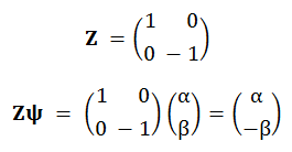
Notice that these four are exactly the states that Alice prepared last time, in the Superdense Coding protocol, by inserting either an X or a Z gate (or both, or neither) into the path of the top qubit of a pair - an entangled pair, which happened to have been prepared in a certain special initial state. We now recognise that state as B₀ = (00+11)/√2.

Exactly as before, it's easy to check by substitution that we can express the Bell state mapping the other way round, for convenience in our subsequent conversions:

00 = (B₀+B₂)/√2,
01 = (B₁-B₃)/√2,
10 = (B₁+B₃)/√2,
11 = (B₀-B₂)/√2.

Partial Measurements

Our third and final new concept of the day is that of a partial measurement. What happens to a composite, multi-qubit state when we perform measurements upon some, but not all, of its constituent qubits? Answer: measured qubits collapse into appropriate basis states in accordance with the probabilities in effect, while unmeasured ones continue in renormalized superpositions.

Take for example the 2-qubit state (a, b, c, d) = a00 + b01 + c10 + d11, and suppose that we perform a measurement, in the computational basis, on its first qubit. Then the probability of getting a result of 0 is simply the sum of the probabilities of getting either 00 or 01 from a full, 2-qubit measurement. Similarly, the probability of a 1 is just the sum for 10 and 11:

prob(0?) = prob(00) + prob(01) = |a|² + |b|²,
prob(1?) = prob(10) + prob(11) = |c|² + |d|².

Okay, that tells us everything we can ever know about the first qubit. What can we say about the posterior state of the second qubit, i.e., its state after this partial measurement? We can answer this by rewriting the original state, collecting terms involving a result of 0 or 1 for the first qubit measurement:

(a, b, c, d) = a00 + b01 + c10 + d11 = 0 (a0 + b1) + 1 (c0 + d1).

This lets us read off the result. If the measurement yielded 0 for the first qubit, then the second qubit is now in the state indicated by a0 + b1, which of course we must renormalize as usual:

(a0 + b1) / √(|a|² + |b|²).

Similarly, a measurement of 1 for the first qubit implies that the second is now in this state:

(c0 + d1) / √(|c|² + |d|²).

Quantum Teleportation

Now we finally have enough background to understand the Quantum Teleportation protocol, which is illustrated in the diagram below. Alice starts with an arbitrary qubit state which I've called ψ, pronounced sigh, out of deference to 86 years of quantum mechanics... sorry about that!

So Alice starts with ψ = (a, b) = a0 + b1, where |a|² + |b|² = 1. This is the state she wants to communicate to Bob; and she also has access to one qubit of an entangled pair, previously prepared in the state

B₀ = (00+11)/√2.

She now performs the "decoding" second half of the Superdense Coding protocol on her two qubits. So that's a cNOT, followed by a Hadamard on the first qubit, then a 2-qubit measurement. Remember, this was the operation performed by Bob last time, and it yields a couple of classical bit results. We've shown these as thick double wires, intended to give the impression of big, strong, macroscopic classical logic levels, insusceptible to decoherence. This decoding operation is actually termed a measurement in the Bell basis. Furthermore, in this setup it's a partial measurement. Recall that we are dealing with a system of three entangled qubits, but measuring only two of them. The third, the bottom one in the diagram, is simply transmitted directly to Bob.


Now Bob examines those two classical bits of data he's received from Alice, and uses them to decide which, if any, of his decoding X and Z gates to apply. His logic is exactly the reverse of the "encoding" step used in the first half of the Superdense Coding protocol. And that's all there is to the Quantum Teleportation protocol; the output that Bob ultimately obtains is identical to Alice's initial, arbitrary state ψ.

I Don't Believe You

And who can blame you! Okay, but be warned: I'll be renormalizing throughout today, so as to avoid any sleight-of-hand accusations. So let's start with the initial state of the 3-qubit system,

(a0 + b1)(00 + 11) / √2 = [a (000 + 011) + b (100 + 111)] / √2.

Alice begins by passing the first two qubits through a cNOT gate. This flips the state of the second qubit in the last two terms, i.e., those where the first "control" qubit is 1, resulting in the state

[a (000 + 011) + b (110 + 101)] / √2.

Next she passes the first qubit through a Hadamard. The effect of this is to replace every initial 0 with (0+1)/√2, and every initial 1 with (0-1)/√2. Collecting terms and combining the √2 divisors, we now have the state

[a (000 + 011 + 100 + 111) + b (001 + 010 - 101 - 110)] / 2.

This is the point at which Alice performs the partial measurement upon the first two qubits. The probability of her getting a result of 00 is

prob(00?) = prob(000) + prob(001) = (|a|² + |b|²) / 4 = ¼,

since |a|² + |b|² = 1. And in fact if you work out the remaining probabilities for results 01, 10 and 11, they all turn out to be ¼. Think about that - the measurement outcome is absolutely random, and completely independent of the particular state of the input qubit ψ! This happens because - thanks to the cNOT and H gates - we are performing the measurement in the Bell basis, and not in the original computational basis where we started.

Fascinating as this detail may be, nevertheless it's not quite what we're after here. We want to know the posterior state of the third qubit. This does depend critically upon the particular 2-bit classical result just obtained, so just as in the Superdense Coding protocol, we now have four distinct cases to consider.

________

Case 00: keeping only the 000 and 001 terms from our state expression and renormalizing, we obtain the state received by Bob:

00 (a0 + b1) = 00 ψ.

That's the magic of quantum teleportation! Without doing anything further, Bob knows from the classical measurement 00 that his third qubit is already in Alice's initial state, ψ.

________

Case 01: keeping only the 010 and 011 terms from our state expression, and renormailzing, we obtain the state received by Bob:

01 (a1 + b0).

Notice however that the 1 bit in the classical measurement result activates the X gate in Bob's decoding circuit, causing a logical inversion of the third qubit, and a final state of

01 (a0 + b1) = 01 ψ.

Again, Bob has successfully received Alice's full state ψ in that third qubit.

________

Case 10: keeping only the 100 and 101 terms from our state expression, and renormailzing, we obtain the state received by Bob:

10 (a0 - b1).

Notice however that the 1 bit in the classical measurement result activates the Z gate in Bob's decoding circuit, causing a sign change in the second basis component of the third qubit, and a final state of

10 (a0 + b1) = 10 ψ.

Again, Bob has successfully received Alice's full state ψ in that third qubit.

________

Case 11: keeping only the 110 and 111 terms from our state expression, and renormailzing, we obtain the state received by Bob:

11 (a1 - b0).

This time both bits in the classical measurement result are 1, so this state becomes subjected to both the full logical inversion and the phase (sign) change, and the final 3-qubit state is

11 (a0 + b1) = 11 ψ.

So in all four cases - in other words, regardless of the outcome of the partial measurement operation - Bob has successfully received Alice's full state ψ in the third qubit.

________

Interactive Demo

Once again Brad Rubin steps up with the Wolfram Demonstrations Project simulation of the Quantum Teleportation protocol, a model of clarity:


This ingenious demo lets you vary both the arbitrary input state ψ, by dragging the indicator point in the upper graph, and the 2-qubit partial measurement result, using the radio buttons below it. Intermediate states of the 3-qubit system are displayed as continuously updated column vectors.

Picture of Star Trek transporter chamber from Wikipedia.

Quantum Computing #4: Superdense Coding

Previously:

Introduction
Single Qubit Gates
Multiple Qubit Gates
Measurement & Review

Note: Last week's removal of Greek lettering and matrices has proved too popular to ignore, all feedback being either positive or neutral, so I'll continue using this "new" notation wherever possible.

Breaking News! A single qubit can transmit two full classical bits of information.

Not on its own, though. We can only ever encode one single classical bit of information into a solitary, unentangled qubit. But when we have access to an entangled pair, we can choose to send one unmodified to our intended recipient, and encode a full two classical bits into the other. To see how, we'll have to examine four quite similar quantum circuits. And we'll need the help of a new single-qubit gate we haven't met before:

The Z Gate

Like its partner the X gate, Z is a kind of inverter. It maps the input qubit state (a, b) to (a, -b). We say that it inverts the phase of the second basis vector. For the sake of completeness alone, here is its matrix representation:

Preparing the Bell State

The two qubits that we'll be using to perform the superdense coding trick have to be entangled, so first let's see how to achieve that. One way is to prepare them both initially in the 0 state. Next, we pass the first qubit of the pair through a Hadamard gate. Finally, we use the output of the H gate as the control input of a controlled-NOT gate, conditionally inverting the second qubit:

The H gate converts the first 0 into 0+1, where I'm going to use '+' and '-' to mean "normalized vector sum" and "normalized vector difference", just to get rid of all the visual noise generated in the calculations by incessant divisions by √2. Since the second qubit remains at 0, the combined state after the H gate is 00+10. Nothing strange about this so far; all it says is that a measurement on the first qubit will yield either 0 or 1, each with 50% probability, while a measurement on the second qubit will still yield 0, with 100% certainty.

Next, the qubits arrive at the cNOT gate. This has no effect upon the first part 00 of the superposition, since there the control (first) qubit is 0. However the second part, 10, has a 1 in the control bit position, causing the cNOT gate to invert the second qubit. The combined state at the output of the cNOT gate is therefore 00+11.

This is termed a Bell State, and it's actually a fairly remarkable state when you think about it. It says that the qubit pair is in a perfectly balanced superposition of the 00 and 11 states. Expressed as a sequence of renormalized amplitudes, it is

(a, b, c, d) = (1/√2, 0, 0, 1/√2)

Since |a|² = |d|² = ½, while |b|² = |c|² = 0, this says that a measurement is equally likely (50%) to yield 00 or 11, and to do so absolutely randomly; but it can never yield 01 or 10. Now if you measure just one of the qubits, whatever result you obtain, 0 or 1, you'll get exactly the same outcome when you measure the second qubit. Even if it's hours or years later, miles or light years away.

Encoding and Decoding

Remember that both Hadamard gates and inverters are their own inverses. If we were to make a mirror image of the above diagram and then join the two together, our final output state would be the same as the originally prepared 00, with probability 100%. This mirror image decoder is shown below, if we temporarily ignore the "?" gate (imagine it to be just a quantum wire, or an Identity gate I):

Suppose Alice is in charge of the "?" box, and Bob is performing the final measurements. Alice wants to send 2 classical bits of data to Bob, but she's only allowed to operate upon the first of the two qubits (the top one in the diagram) to do it. What should she put in the "?" box?

Well, if the bits she wants to send are 00, then she need apply nothing but a simple quantum wire, since we've just seen that this will result in Bob's measurements yielding the result 00 with 100% certainty. In the more general case, she needs to examine both of the classical bits that she wants to send. If the first is 1, then she should add our new friend the Z gate in place of the "?". If the second is 1, she adds an X. Note that if both bits are 1, she will now have added both a Z and a following X.

00 → I
01 → Z
10 → X
11 → Z followed by X

And that's all there is to the Superdense Coding Protocol. With those arrangements in place, Bob's measurements will always yield, with 100% certainty, the particular combined state 00, 01, 10, or 11 that Alice wanted to send him.

I Don't Believe You

No, you'd be mad to, unless you're already a QC expert! We'll go through the four cases individually in detail. Remember, the starting point for Alice is in each case the Bell State 00+11. It will also be useful to remember the reversibility of the H gate. Just as it converts basis states 0 and 1 respectively into their sum 0+1 and difference 0-1, so when presented with a sum 0+1 at its input, does it output 0; and with a difference 0-1, output 1.

Case 00: We already established, using an argument based on considerations of symmetry, the correct operation of the circuit for this first case. Still, it's worth running through the detailed sequence of decoding steps, since these are the same for all subsequent cases. So: Alice does nothing to the 00+11 state, which is then passed immediately into the second cNOT gate. This has no effect on the 00 portion of its input, but changes the 11 part (because the first, control bit is 1) into 10. The cNOT output is therefore 00+10. The first of these qubits, 0+1, is fed to the second Hadamard, which as mentioned above, converts it to 0. Therefore, the final 2-qubit output is 00, with probability 100%.

Case 01: Alice inserts an X gate in the path of the first qubit, converting the initial 00+11 to 10+01. The cNOT changes this to 11+01, feeding the first qubit 1+0 into H, which outputs 0. Therefore, the final 2-qubit output is 01, with probability 100%.

Case 10: Alice inserts a Z gate in the path of the first qubit, converting the initial 00+11 to 00-11. The cNOT changes this to 00-10, feeding the first qubit 0-1 into H, which outputs 1. Therefore, the final 2-qubit output is 10, with probability 100%.

Case 11: Alice inserts both a Z and a following X into the path of the first qubit, converting the initial 00+11 first to 00-11 as in the previous case, then to 10-01. The cNOT changes this to 11-01, feeding the first qubit 1-0 into H, which outputs 1. Therefore, the final 2-qubit output is 11, with probability 100%.

Quantum Erat Demonstrandum!

The second most surprising thing about Superdense Coding - other than the fact that in reality, it works exactly as advertised! - is the time it took to get itself discovered. The whole subject of Quantum Mechanics was kicked off by Werner Heisenberg in 1925, with Quantum Computing eventually appearing with Richard Feynman in 1982; yet it was a further ten years after that before the definitive Bennett & Wiesner paper appeared, noting that certain "EPR" (Einstein-Podolsky-Rosen) states "allow two bits to be encoded reliably in one spin-½ particle..."

Interactive Demo

The Wolfram Demonstrations Project contains a great interactive demo of the Superdense Coding protocol, one of several contributed by Brad Rubin. This varies a little from the our example, specifically in the order of the X and Z gates during the 11 case, but the difference vanishes during final measurement. You interact with it by downloading the Computable Document Format (CDF) Player, and optionally the Superdense Coding demo file itself, which looks like this:


As you can see, it displays all the intermediate states of the qubits during this quantum computation - and fully normalized, hence all the "1/√2"s.

Footnote

In this series I've been avoiding discussion about the physical realisation of qubits, but the day after I posted this comment on digital simulator Logicly's Facebook page...

Has anyone ever asked for a quantum circuit version? You seem to have all the component building and layout logic that would require. Qubit signals: rather than boolean, these would be pairs of complex numbers (or quadruples of floats), and there would be a "measurement" gate with a classical boolean 0 or 1 output. Now seems a good time to start training up on these!

... noted futurologist and SF author Charles Stross predicted room temperature quantum computing on integrated circuitry within 5 to 20 years, based on a fascinating discovery about silicon carbide. My guess is that many more suitable materials will be discovered quite soon, making available QC technologies that will have absolutely no trouble attracting capital investment at the left hand edge of that range.

Next time: Quantum Teleportation.

My Work in Print: 1985

I've previously written about the very competitive crafting of optimum machine code programs for Personal Computer World magazine's 1980s Sub Set series, here and there. In 1985, the incumbent series editor David Barrow convinced Century Communications to publish two books of the best submissions. According to the descriptions on their publication history pages, these books were "Edited and produced working directly from the author's word-processor by NWL Editorial Services, Rushley, High Ham, Somerset" - a huge novelty in the publishing world at the time. Book geeks: note the cool adjacent ISBNs!

Best of PCW Assembler Routines for the Z80

Although the first IBM PC with its 8-bit Intel 8088 chip had already been available for about four years, still most business software was based on the CP/M operating system, and the more powerful, backward compatible Zilog Z80. Joined to legion Sinclair hobbyists, these users constituted quite an army. Here is the index of my contributions to the Z80 edition:

• ECAL - Calculate error correction byte; pp. 70-71.
• EFIX - Validate data with error correction byte; pp. 71-72.
• NEWPC - Anticipate PC contents after next instruction; pp. 78-82.
• RDM32 - 32-bit pseudo-random number generator; pp. 147-149.
• SQR31 - Square root of 32-bit signed (positive) value; pp. 169-170.
• SQR32 - Square root of 32-bit unsigned (absolute) value; pp. 169-170.
• CURT16 - Cube Root of a 16-bit unsigned integer value; pp. 170-174.
• CURT32 - Cube Root of a 32-bit unsigned integer value; pp. 174-176.
• SDIV4 - 4-byte signed integer division; pp. 183-185.

Barrow, David (editor)
Best of Personal Computer World Assembler Routines for the Z-80
Century Communications Ltd
1985
ISBN 0 7126 0506 1

Best of PCW Assembler Routines for the 6502

While businessmen cycled their Z80s, many hobbyists with an aversion to dead-flesh rubber keyboards were devouring Commodore VIC-20s and 64s, and Acorn's BBC Micro. All of these used the MOS Technology 6502 processor. Here is the index of my contributions to the 6502 edition:

• RINXY - Register Indirect addressing mode emulator; pp. 20-22.
• ECAL - Calculate error correction byte; pp. 88-90.
• EFIX - Validate data with error correction byte; pp. 90-91.
• SQR15 - Square root of 16-bit signed (positive) value; pp. 125-127.
• SQR16 - Square root of 16-bit unsigned (absolute) value; pp. 125-127.
• SQR31 - Square root of 32-bit signed (positive) value; pp. 127-129.
• SQR32 - Square root of 32-bit unsigned (absolute) value; pp. 127-129.
• CURT16 - Cube Root of a 16-bit unsigned integer value; pp. 129-134.
• CURT32 - Cube Root of a 32-bit unsigned integer value; pp. 134-137.

Barrow, David (editor)
Best of Personal Computer World Assembler Routines for the 6502
Century Communications Ltd
1985
ISBN 0 7126 0507 X

A Disassembler in ~1KB

Colleague C keeps reminding me that The SUBSET editor David Barrow was able to trim only one byte from John Kerr's compact code. What the hell is he talking about? The quote comes from this ZX Spectrum Utility, whose author explains: The stated aim was to write a Z80 disassembly routine in as short a space as possible and, at just over 1K (1090 bytes), it is a rather incredible program.

Unfortunately my DISZ80 routine was submitted too late - by about two years - for inclusion in the book, and I no longer have the magazine that it appeared in. At the risk of sounding a bit JR Hartley, if anyone out there has that 1987 issue, it would be good to be able to restore the line comments to the utility. I work in self-documenting, high level languages now, eschewing comments almost universally. But part of the strict Sub Set documentation standard insisted that every single machine code instruction got fully commented. Oh, and it would also be nice to see exactly where Dave Barrow's one-byte optimization appeared!

[Update 30 April 2012: This has now been done, many thanks to my new best friends Geoff Wearmouth and Stephen Parry-Thomas! See comments below, and also My Work in Print: 1987]

Cube Root Algorithm

I derived the method of cube root extraction used in both books, by applying a kind of induction by analogy to the existing square root algorithm. Dave thought my description of the process sufficiently interesting to publish it. Click for readability:



Next time: 1987

Algebra of Functions, Part 4: Parsers

A Series of Tubes

Note: this 2010 series of articles (part one, two, three, 3½) was abandoned incomplete when overtaken by events at the Microsoft C# compiler factory. My utimate target, actually intended to be the article right after this one, was the Continuation Monad; but Eric Lippert got there before me with a surprise sprint (Continuation Passing Style Revisited, part one, two, three, four, five) leading up to his introduction to async/await marathon (Asynchrony in C# 5, part one, two, three, four, five, six, seven, eight). The only reason to publish this short excerpt now is to have a convenient index into the work of Brian McNamara and Luke Hoban, as linked at the end.

Today we take a look at another popular exhibit from the monad menagerie: the Parse monad.

Parsing is such a popular example of the application of monads, because it so neatly fits the characteristic template of a data processing pipeline with side effects. When parsing a string into any given language, each successive step

1. consumes part of the input string, and then
2. passes the remainder on to the next step in the sequence.
   

That constitutes the main process. But as a side effect, the just-parsed value is also made available in some way. This might be a keyword of the language, the name of a variable, or perhaps a binary value representing a data value of some particular type; but it could equally well be discardable whitespace, or any character, etc.

In terms of our monad then, the unamplified type is the input type string. The amplified type, which must be capable of holding all of the output from an operation of parsing, needs to store both a string, representing the remainder of the unconsumed input, and another, parsed value, of some arbitrary type.

Language geeks love all monads and parser combinators in equal measure, and there is a wealth of information about all this stuff on the web. As for C#, one of the best and most detailed I've seen is Brian McNamara's December 2007 series, "Monadic Parser Combinators", which gets as far as Part Eight before surrendering to F#:

Part: One, Two, Three, Four, Five, Six, Seven, Eight.
Source: Part 4, Part 5/6.

Very succinct and readable is Luke Hoban's contribution, also from 2007:

Monadic Parser Combinators using C# 3.0